import numpy as np
import pandas as pd
import matplotlib.pyplot as plt
import sklearn.linear_model선형회귀분석의 시작 | LinearRegression()
linear_model
sklearn의linear_mode.LinearRegression()을 사용하여 선형회귀분석을 해보자!
해당 포스트는 전북대학교 통계학과 최규빈 교수님의 강의내용을 토대로 재구성되었음을 알립니다.
1. 라이브러리 imports
2. Data
전주시의 기온 자료
temp = pd.read_csv('https://raw.githubusercontent.com/guebin/DV2022/master/posts/temp.csv').iloc[:,3].to_numpy()[:100]
temp.sort() ## 자료를 크기 순서대로 정렬, sort_values()와 비슷하달까...temparray([-4.1, -3.7, -3. , -1.3, -0.5, -0.3, 0.3, 0.4, 0.4, 0.7, 0.7,
0.9, 0.9, 1. , 1.2, 1.4, 1.4, 1.5, 1.5, 2. , 2. , 2. ,
2.3, 2.5, 2.5, 2.5, 2.6, 2.6, 2.9, 3.2, 3.5, 3.5, 3.6,
3.7, 3.8, 4.2, 4.4, 4.5, 4.5, 4.6, 4.9, 4.9, 4.9, 5. ,
5. , 5.1, 5.6, 5.9, 5.9, 6. , 6. , 6.1, 6.1, 6.3, 6.3,
6.4, 6.4, 6.5, 6.7, 6.8, 6.8, 7. , 7. , 7.1, 7.2, 7.4,
7.7, 8. , 8.1, 8.1, 8.3, 8.4, 8.4, 8.4, 8.5, 8.8, 8.9,
9.1, 9.2, 9.3, 9.4, 9.4, 9.5, 9.6, 9.6, 9.7, 9.8, 9.9,
10.2, 10.3, 10.6, 10.6, 10.8, 11.2, 12.1, 12.4, 13.4, 14.7, 15. ,
15.2])- 아래와 같은 모형을 가정하자. \[\textup{아이스크림 판매량}= 20 + \textup{온도} × 2.5 × \textup{오차(운)}\]
- 더미 모형 생성
np.random.seed(43052)
eps = np.random.randn(100)*3  ## 오차
icecream_sales = 20 + temp * 2.5 + eps
plt.plot(temp, icecream_sales, 'o')
plt.show()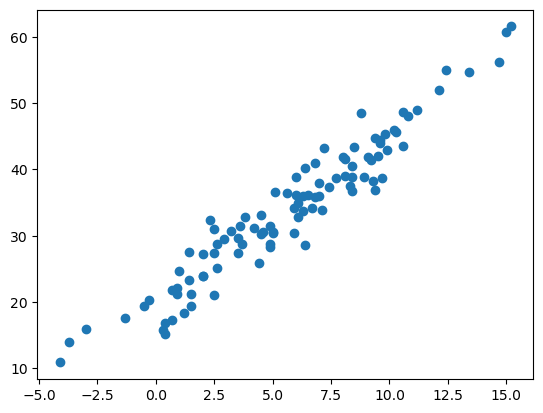
상기 결과를 관측했다고 생각합시다.
df = pd.DataFrame({'temp' : temp, 'sales' : icecream_sales})
df| temp | sales | |
|---|---|---|
| 0 | -4.1 | 10.900261 |
| 1 | -3.7 | 14.002524 |
| 2 | -3.0 | 15.928335 |
| 3 | -1.3 | 17.673681 |
| 4 | -0.5 | 19.463362 |
| ... | ... | ... |
| 95 | 12.4 | 54.926065 |
| 96 | 13.4 | 54.716129 |
| 97 | 14.7 | 56.194791 |
| 98 | 15.0 | 60.666163 |
| 99 | 15.2 | 61.561043 |
100 rows × 2 columns
3. 게임세팅
- 편의상 아래와 같은 기호를 도입하자.
- (
df.temp[0],df.temp[1], … ,df.temp[99]) = \((x_1,x_2,\dots,x_{100})=(-4.1,-3.7,\dots,15.2)\) - (
df.sales[0],df.sales[1], … ,df.sales[99]) = \((y_1,y_2,\dots,y_{100})=(10.90,14.00, \dots,61.56)\)
이 자료 \(\big\{(x_i,y_i)\big\}_{i=1}^{100}\)를 바탕으로 어떠한 패턴을 발견하여 새로운 \(x\)에 대한 예측값을 알고 싶다 : \(\hat{y}\)
A. 질문
- 기온이 \(x = -2.0\)일 때, 아이스크림을 얼마정도 판다고 보는 게 타당할까?
B. 답 1
- \(x = -2.0\) 근처의 데이터를 살펴보자.
df[(-4.0 < df.temp) & (0.0 > df.temp)]| temp | sales | |
|---|---|---|
| 1 | -3.7 | 14.002524 |
| 2 | -3.0 | 15.928335 |
| 3 | -1.3 | 17.673681 |
| 4 | -0.5 | 19.463362 |
| 5 | -0.3 | 20.317853 |
\(-1.3\)이 제일 가까운데, 대충 \(17.67\) 언저리 아닐까…?
A. 산점도와 추세선
- 자료를 바탕으로 그림을 그려보자
plt.plot(df.temp, df.sales, 'o')
plt.plot([-2.0],[17.67],'x')     # 이미 들어가있는 플롯에 점을 하나 찍는다. 마커는 X

plt.show()
예상한 것(17.67)보다 못팔 것 같은데…?
### B. 아이디어
- 선을 기가 막히게 그어서 추세선을 만들고, 그 추세선 위의 점으로 예측하자!~(사실 모형을 우리가 만들었으니 이미 추세선을 알고 있긴 함)~
plt.plot(df.temp, df.sales, 'o')
plt.plot(df.temp, 20+df.temp*2.5, '--')  ## 위에서 직접 설정했던 자료의 관계, 절편이 20이고 기울기가 2.5

plt.show()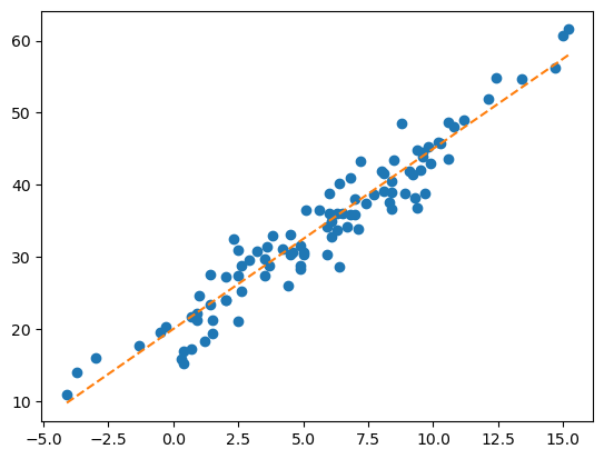
- 사실 \(y = 20 + 2.5x\)라는 추세선을 이미 알고 있었음.
- 그래서 \(x = -2\)라면 \(y = 20 - 2.5 × 2 = 15\)라고 보는 게 합리적임(오차를 고려 안하면)
허나, 실제 상황에서 우리는 \(20, 2.5\)라는 숫자를 모른다.
- 게임셋팅 * 원래 게임 : 임의의 \(x\)에 대하여 합리적인 \(y\)를 잘 찾는 게임 * 변형된 게임 : \(20, 2.5\)라는 숫자를 잘 찾는 게임. 즉, 데이처를 보고 최대한 \(y_i \approx ax_i+b\)가 되도록 \(a, b\)를 잘 선택하는 게임
4. 분석
그렇다면 늘 했던 것처럼 네 단계로 분석을 해보자.
A. 데이터
# step 1 -- data
train = pd.DataFrame({'temp' : temp, 'sales' : icecream_sales})

X = train[['temp']]
y = train['sales']
데이터를 학습해서 추세선을 적절히 그릴 수 있고, 그려진 추세선으로 예측까지 해줄 수 있는 아이(predictor)를 만들자.~(근데 이정도면 학생이 아니라 노예…)~
### B. predictor
# step 2
predictr = sklearn.linear_model.LinearRegression()
sklearn의linear_model.LinearRegression()을 사용했다. 이러면 가장 기본적인 선형회귀를 진행한다.(LSE를 쓰는 그거 있잖아…)
C. 학습
# step 3
predictr.fit(X, y)LinearRegression()In a Jupyter environment, please rerun this cell to show the HTML representation or trust the notebook.
On GitHub, the HTML representation is unable to render, please try loading this page with nbviewer.org.
LinearRegression()
학생이 train을 완료했다.
### D. 예측(predict)
- 학생(predictr) : 데이터를 살펴보니 True는 이럴 것 같아요.
y_hat = predictr.predict(X) ## X값에 해당하는 y_hat값을 예측하여 산출.plt.plot(X, y, 'o', alpha = 0.5)
plt.plot(X, y_hat, 'o--', alpha = 0.5)
plt.show()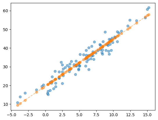
- 그럼 기울기와 절편은 어디에 저장된 걸까?
- predictr : 여깄음.
(predictr.coef_, predictr.intercept_)(array([2.51561216]), 19.66713126947925)- 새로운 데이터 \(x = -2\)에 대한 예측
float(predictr.coef_)*(-2) + float(predictr.intercept_)14.63590694951262해당 결과값을 그래프에 나타내면…
X_input = pd.DataFrame({'temp' : [-2.0]})plt.plot(X, y, 'o', alpha = 0.5)
plt.plot(X, y_hat, '--', alpha = 0.5)
plt.plot(X_input, predictr.predict(X_input), 'xr') ## 원래는 리스트나 어레이로 넣어주는 게 정배긴 함
plt.show()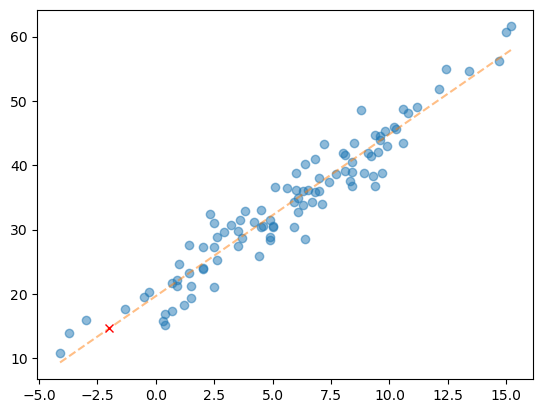
예측값이 직선상에 위치함을 알 수 있다.
5. 두 타입의 아이스크림(초코 / 바닐라)에 대한 회귀분석
이전의 기온 자료를 바꿔 아래와 같은 모형을 가정해보자.
A. Data
temp = pd.read_csv('https://raw.githubusercontent.com/guebin/DV2022/master/posts/temp.csv').iloc[:,3].to_numpy()[:100]
temp.sort()   ## 자료를 크기 순서대로 정렬
temp  ## 전주시의 기온 100개 자료
array([-4.1, -3.7, -3. , -1.3, -0.5, -0.3, 0.3, 0.4, 0.4, 0.7, 0.7,
0.9, 0.9, 1. , 1.2, 1.4, 1.4, 1.5, 1.5, 2. , 2. , 2. ,
2.3, 2.5, 2.5, 2.5, 2.6, 2.6, 2.9, 3.2, 3.5, 3.5, 3.6,
3.7, 3.8, 4.2, 4.4, 4.5, 4.5, 4.6, 4.9, 4.9, 4.9, 5. ,
5. , 5.1, 5.6, 5.9, 5.9, 6. , 6. , 6.1, 6.1, 6.3, 6.3,
6.4, 6.4, 6.5, 6.7, 6.8, 6.8, 7. , 7. , 7.1, 7.2, 7.4,
7.7, 8. , 8.1, 8.1, 8.3, 8.4, 8.4, 8.4, 8.5, 8.8, 8.9,
9.1, 9.2, 9.3, 9.4, 9.4, 9.5, 9.6, 9.6, 9.7, 9.8, 9.9,
10.2, 10.3, 10.6, 10.6, 10.8, 11.2, 12.1, 12.4, 13.4, 14.7, 15. ,
15.2])- 아래와 같은 모형을 가정하자.
\[\textup{초코 아이스크림 판매량} = 20 + \textup{온도} \times 2.5 + \textup{오차(운)}\]
\[\textup{바닐라 아이스크림 판매량} = 40 + \textup{온도} \times 2.5 + \textup{오차(운)}\]
np.random.seed(43052)
choco = 20 + temp*2.5 + np.random.randn(100)*3  ## random normal distribution
vanilla = 40 + temp*2.5 + np.random.randn(100)*3
plt.plot(temp, choco, 'o', label = 'choco')
plt.plot(temp, vanilla, 'o', label = 'vanilla')
plt.legend()
plt.show()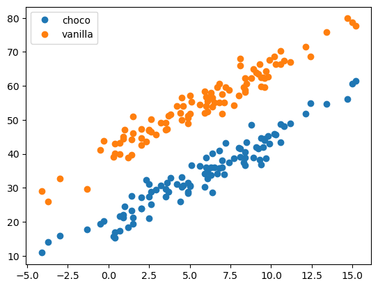
우리는 위와 같은 정보를 관측했다고 가정하자.
df1 = pd.DataFrame({'temp' : temp, 'type' : ['choco' for i in range(100)], 'sales' : choco})
df2 = pd.DataFrame({'temp' : temp, 'type' : ['vanilla' for i in range(100)], 'sales' : vanilla})

df = pd.concat([df1, df2], axis = 0).reset_index(drop = True)
df| temp | type | sales | |
|---|---|---|---|
| 0 | -4.1 | choco | 10.900261 |
| 1 | -3.7 | choco | 14.002524 |
| 2 | -3.0 | choco | 15.928335 |
| 3 | -1.3 | choco | 17.673681 |
| 4 | -0.5 | choco | 19.463362 |
| ... | ... | ... | ... |
| 195 | 12.4 | vanilla | 68.708075 |
| 196 | 13.4 | vanilla | 75.800464 |
| 197 | 14.7 | vanilla | 79.846568 |
| 198 | 15.0 | vanilla | 78.713140 |
| 199 | 15.2 | vanilla | 77.595252 |
200 rows × 3 columns
### B. 분석
- 언제처럼 늘 그랬던 것처럼…
# step 1
## X = pd.get_dummies(df).drop(['sales'], axis = 1) ## 이게 제일 범용적이긴 함
X = df.loc[:, ['temp', 'type']].assign(type = (df.type == 'choco')) ## 직관적으로 쓴 코드, 범주형은 인식을 못한다.
y = df['sales']

# step 2
predictr = sklearn.linear_model.LinearRegression()

# step 3
predictr.fit(X, y)

# step 4
df = df.assign(sales_hat = predictr.predict(X));df| temp | type | sales | sales_hat | |
|---|---|---|---|---|
| 0 | -4.1 | choco | 10.900261 | 9.286731 |
| 1 | -3.7 | choco | 14.002524 | 10.295689 |
| 2 | -3.0 | choco | 15.928335 | 12.061366 |
| 3 | -1.3 | choco | 17.673681 | 16.349439 |
| 4 | -0.5 | choco | 19.463362 | 18.367355 |
| ... | ... | ... | ... | ... |
| 195 | 12.4 | vanilla | 68.708075 | 71.446479 |
| 196 | 13.4 | vanilla | 75.800464 | 73.968875 |
| 197 | 14.7 | vanilla | 79.846568 | 77.247989 |
| 198 | 15.0 | vanilla | 78.713140 | 78.004708 |
| 199 | 15.2 | vanilla | 77.595252 | 78.509187 |
200 rows × 4 columns
- 가장 중요한 시각화까지…
plt.plot(df.temp, df.sales, 'o')
plt.plot(df.loc[df.type == 'choco'].temp, df.loc[df.type == 'choco'].sales_hat, '--', color = 'brown', label = 'choco')
plt.plot(df.loc[df.type == 'vanilla'].temp, df.loc[df.type == 'vanilla'].sales_hat, '--', color = 'yellow', label = 'vanilla')
plt.legend()
plt.show()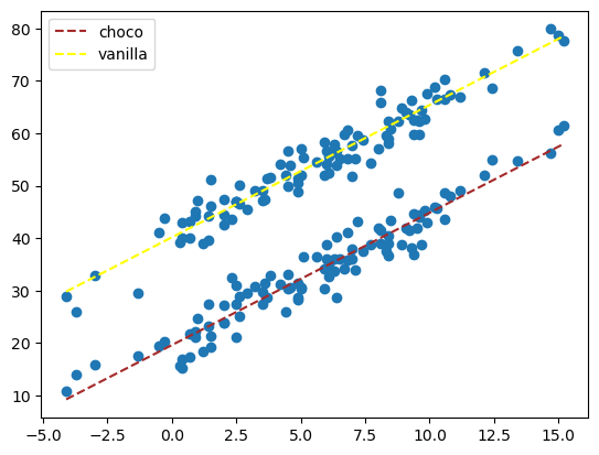
별다른 뜻 없이 (초코, 바닐라)에 (1, 0)을 넣었는데, 어떻게 뭐가 나오긴 했다.
어케했음???
\[\textup{아이스크림 판매량} = 40 + \textup{아이스크림종류} \times (-20) + \textup{온도} \times 2.5 + \textup{오차(운)}\]
predictr.coef_, predictr.intercept_(array([ 2.52239574, -20.54021854]), 40.16877158069265)coef_(기울기)가 2개지요.
온도와 범주형 자료인 아이스크림 종류에 따라 기울기가 다르다. 온도 1도가 변할때마다 판매량은 2.52239574가 변하고, 아이스크림 종류가 1 변할때마다(0에서 1이니까 바닐라에서 초코로 바뀜) -20.54를 곱한 수를 더하여 수식을 설명하였다.
예측
- 온도가 \(-2\)이고, type이 vanilla(0)라면 예측값은?
Xnew = pd.DataFrame({'temp' : [-2], 'type' : [0]})

predictr.predict(Xnew)array([35.1239801])plt.plot(df.temp, df.sales, 'o')
plt.plot(df.loc[df.type == 'choco'].temp, df.loc[df.type == 'choco'].sales_hat, '--', color = 'brown', label = 'choco')
plt.plot(df.loc[df.type == 'vanilla'].temp, df.loc[df.type == 'vanilla'].sales_hat, '--', color = 'yellow', label = 'vanilla')
plt.plot(Xnew.temp, predictr.predict(Xnew), 'or', label = 'prediction')
plt.legend()
plt.show()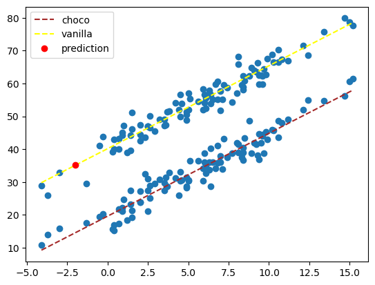
C. 데이터 전처리
- 아까 pd.get_dummies()를 잠시 본 것 같은데, 이걸 어떻게, 왜 써야 하는 지 알아보자.
X = df[['temp','type']] # 독립변수, 설명변수, 피쳐
y = df[['sales']] # 종속변수, 반응변수, 타겟
X = pd.get_dummies(X);X| temp | type_choco | type_vanilla | |
|---|---|---|---|
| 0 | -4.1 | True | False |
| 1 | -3.7 | True | False |
| 2 | -3.0 | True | False |
| 3 | -1.3 | True | False |
| 4 | -0.5 | True | False |
| ... | ... | ... | ... |
| 195 | 12.4 | False | True |
| 196 | 13.4 | False | True |
| 197 | 14.7 | False | True |
| 198 | 15.0 | False | True |
| 199 | 15.2 | False | True |
200 rows × 3 columns
원-핫 인코딩 : 표현하고 싶은 단어에는 1을, 그것이 아닌 것에는 0을 부여
- LinearRegression 모델의 경우 범주형 자료를 자동으로 인식하지 못한다. 따라서 구분할 범주형 변수가 많다면, pd.get_dummies()를 통해 범주를 나눠주어야 한다.
### D. 모형의 평가
- 단순선형회귀분석의 경우 모형을 \(R^2\)(결정계수)로 평가한다.
다만 이것이 높다고 해서 무조건적으로 좋은 건 아니고, 명확한 기준도 없다. 모형 간 상대적인 좋음을 비교하는 것 뿐이다.
- LogisticRegression에서는 적중률로 딱 떨어지게 점수를 내줄 수 있겠지만, 이건 그렇게 해버리면 0점이 나와버리겠지…
6. 설명변수가 많을 때
- kaggle에서 “Medical Cose Personal Datasets”을 다운로드
https://www.kaggle.com/datasets/mirichoi0218/insurance
df = pd.read_csv(".\data\insurance.csv")
df| age | sex | bmi | children | smoker | region | charges | |
|---|---|---|---|---|---|---|---|
| 0 | 19 | female | 27.900 | 0 | yes | southwest | 16884.92400 |
| 1 | 18 | male | 33.770 | 1 | no | southeast | 1725.55230 |
| 2 | 28 | male | 33.000 | 3 | no | southeast | 4449.46200 |
| 3 | 33 | male | 22.705 | 0 | no | northwest | 21984.47061 |
| 4 | 32 | male | 28.880 | 0 | no | northwest | 3866.85520 |
| ... | ... | ... | ... | ... | ... | ... | ... |
| 1333 | 50 | male | 30.970 | 3 | no | northwest | 10600.54830 |
| 1334 | 18 | female | 31.920 | 0 | no | northeast | 2205.98080 |
| 1335 | 18 | female | 36.850 | 0 | no | southeast | 1629.83350 |
| 1336 | 21 | female | 25.800 | 0 | no | southwest | 2007.94500 |
| 1337 | 61 | female | 29.070 | 0 | yes | northwest | 29141.36030 |
1338 rows × 7 columns
A. 분석
열 이름을 먼저 알아보자.
set(df.columns){'age', 'bmi', 'charges', 'children', 'region', 'sex', 'smoker'}df.info()<class 'pandas.core.frame.DataFrame'>
RangeIndex: 1338 entries, 0 to 1337
Data columns (total 7 columns):
# Column Non-Null Count Dtype
--- ------ -------------- -----
0 age 1338 non-null int64
1 sex 1338 non-null object
2 bmi 1338 non-null float64
3 children 1338 non-null int64
4 smoker 1338 non-null object
5 region 1338 non-null object
6 charges 1338 non-null float64
dtypes: float64(2), int64(2), object(3)
memory usage: 73.3+ KB- 대충 여러가지 범주형ㆍ연속형 설명변수들과 보험료의 관계를 요약하고 싶다고 하자.
먼저 범주형 자료(
sex,smoker,region)들을 원-핫 인코딩 해주자.
X = pd.get_dummies(df.drop(['charges'], axis = 1))
y = df.charges

X| age | bmi | children | sex_female | sex_male | smoker_no | smoker_yes | region_northeast | region_northwest | region_southeast | region_southwest | |
|---|---|---|---|---|---|---|---|---|---|---|---|
| 0 | 19 | 27.900 | 0 | True | False | False | True | False | False | False | True |
| 1 | 18 | 33.770 | 1 | False | True | True | False | False | False | True | False |
| 2 | 28 | 33.000 | 3 | False | True | True | False | False | False | True | False |
| 3 | 33 | 22.705 | 0 | False | True | True | False | False | True | False | False |
| 4 | 32 | 28.880 | 0 | False | True | True | False | False | True | False | False |
| ... | ... | ... | ... | ... | ... | ... | ... | ... | ... | ... | ... |
| 1333 | 50 | 30.970 | 3 | False | True | True | False | False | True | False | False |
| 1334 | 18 | 31.920 | 0 | True | False | True | False | True | False | False | False |
| 1335 | 18 | 36.850 | 0 | True | False | True | False | False | False | True | False |
| 1336 | 21 | 25.800 | 0 | True | False | True | False | False | False | False | True |
| 1337 | 61 | 29.070 | 0 | True | False | False | True | False | True | False | False |
1338 rows × 11 columns
- 그럼 뭐 늘 하던대로…
# 2
predictr = sklearn.linear_model.LinearRegression()

# 3
predictr.fit(X, y)

# 4
df = df.assign(y_hat = predictr.predict(X))df| age | sex | bmi | children | smoker | region | charges | y_hat | |
|---|---|---|---|---|---|---|---|---|
| 0 | 19 | female | 27.900 | 0 | yes | southwest | 16884.92400 | 25293.713028 |
| 1 | 18 | male | 33.770 | 1 | no | southeast | 1725.55230 | 3448.602834 |
| 2 | 28 | male | 33.000 | 3 | no | southeast | 4449.46200 | 6706.988491 |
| 3 | 33 | male | 22.705 | 0 | no | northwest | 21984.47061 | 3754.830163 |
| 4 | 32 | male | 28.880 | 0 | no | northwest | 3866.85520 | 5592.493386 |
| ... | ... | ... | ... | ... | ... | ... | ... | ... |
| 1333 | 50 | male | 30.970 | 3 | no | northwest | 10600.54830 | 12351.323686 |
| 1334 | 18 | female | 31.920 | 0 | no | northeast | 2205.98080 | 3511.930809 |
| 1335 | 18 | female | 36.850 | 0 | no | southeast | 1629.83350 | 4149.132486 |
| 1336 | 21 | female | 25.800 | 0 | no | southwest | 2007.94500 | 1246.584939 |
| 1337 | 61 | female | 29.070 | 0 | yes | northwest | 29141.36030 | 37085.623268 |
1338 rows × 8 columns
- charge와 y_hat이 잘 안맞는 것 같은데…?
### B. 평가
predictr.score(X, y)0.7509130345985205\(R^2 = \frac{SSR}{SST} = 0.7509130345985205\)
0.7 이상이면 망한 모형까진 아니지만…
계수 해석
- 상수항
predictr.intercept_-666.9377199366372기본적인 보험료(다른 모든 것이 0일 때)는 -666이다.~(딱봐도 이상하죠? 그래서 별로 의미는 없다.)~
- 계수
pd.DataFrame({'columns' : X.columns, 'coef' : predictr.coef_})| columns | coef | |
|---|---|---|
| 0 | age | 256.856353 |
| 1 | bmi | 339.193454 |
| 2 | children | 475.500545 |
| 3 | sex_female | 65.657180 |
| 4 | sex_male | -65.657180 |
| 5 | smoker_no | -11924.267271 |
| 6 | smoker_yes | 11924.267271 |
| 7 | region_northeast | 587.009235 |
| 8 | region_northwest | 234.045336 |
| 9 | region_southeast | -448.012814 |
| 10 | region_southwest | -373.041756 |
- 연속형 : 나이, bmi, 자녀의 수가 많을수록 보험료는 올라갔다.
- 범주형 : 여성, 흡연자의 경우 보험료가 더 비쌌다.
- 지역은 잘 모르겠으나, 나머지는 꽤 그럴듯해 보인다.(지역에 대한 정보는 알기 어려움…)